


⚠️ This is a record attempt, built on other people's work. It's submitted as PR #396 (the code) and PR #397 (the runs), and both are in review. It only becomes a record if the maintainers verify it on their own hardware. The numbers below are from my own runs on one 8×H100 node rented from runpod.io.
Two weeks ago I made my first modded-nanogpt attempt (34.9 seconds, #391). Since then the bar has moved: #393 by Francesco Prignano brought the record to 31.29 seconds with a mixture of experts and custom GPU kernels.
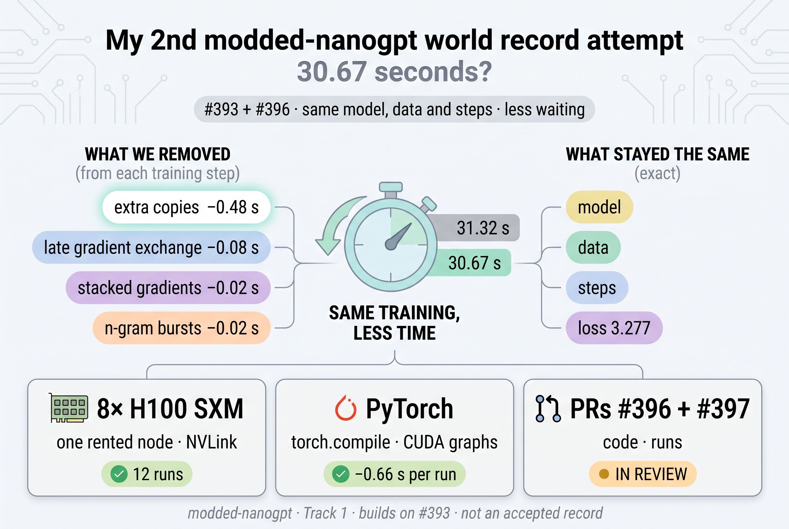
This time I added four improvements to #393's training step, each based on profiling #393 on 8×H100: no extra copies around FlashAttention (17 copy kernels per step), an earlier start for the GPUs' gradient exchange, gradients written in place, and n-gram updates spread evenly over the steps. Together they bring the time to 30.67 seconds, about 0.66 seconds faster than #393's own code on the same machine, with the same model, data and number of steps.
Standing on other people's work
Everything in this attempt is #393's model, data, schedule and step count. The code is in #396 (four small changes, 8 files), and the runs and logs are in #397.
The four improvements
1. No extra copies around FlashAttention (about −0.48 s). #393's fused QKV kernel returns q, k and v as [tokens, heads, dim]. They got a batch dimension added and then immediately removed again before FlashAttention:
# before (#393)
q, k, v = q[None], k[None], v[None]
...
y = flash_attn_varlen_func(q[0], k[0], v[0], cu_seqlens_q=seqlens, ...)

# after (#396): hand the kernel's tensors to FlashAttention as they are
y = flash_attn_varlen_func(q, k, v, cu_seqlens_q=seqlens, ...)
In the forward pass this costs nothing. In the backward pass, though, PyTorch has to undo the [0] selection, and it does that by writing each gradient into a fresh buffer. That is one extra copy kernel after every attention layer, 17 per step. This is most of the gain.
2. Send gradients sooner (about −0.08 s). After the backward pass, the 8 GPUs exchange gradients (reduce-scatter). That exchange used to be queued behind some unrelated gradient copies. Now it starts as soon as the gradients exist, and runs alongside the remaining compute:
def backward(self, launch_reduces=None):
    cs.backward.replay()
    for p, grad in cs.anvil_grads:
        p.grad = grad
    if launch_reduces is not None:
        launch_reduces()   # start the GPUs' gradient exchange now ...
    ...                    # ... instead of after these Adam gradient copies
3. Write gradients in place (about −0.02 s). The dense MLP weight gradients were stacked into their bank, with zero-filled padding slots. They are now written straight into a persistent buffer, as #393 already does for the MoE experts.
4. Spread the n-gram update (about −0.02 s). Every fourth step, #393 applied the gradients of the large n-gram table in one burst. Each step now adds its share right away.
All four are exact: the same kernels compute the same values, so the runs vary only as much as #393's own runs do. EXACT_LEVERS=none switches them all off again.
The numbers
All runs were on one 8×H100 node, with #393's own code timed alongside:
| runs | time | validation loss | |
|---|---|---|---|
| this attempt (#393 + #396) | 12 | 30.67 s | 3.2774 |
| #393, same node | 6 | 31.32 s | 3.2771 |
- Paired seeds: across five seed pairs, the difference is −0.66 s ± 0.05 (t = 31).
- Loss: the 12 runs pass the loss requirement on their own (mean below 3.28 at p < 0.01, t = 7.7).
- Every run counts. I planned 10 runs and extended to 12 before the extra runs started, to match #393's run count.
One finding of my own
Along the way I also tried parameter golf's LeakyReLU² activation on #393. It helped a lot on my Mac, but gave nothing on 8×H100, and it made each run 0.4 s slower.
The reason surprised me. Later in training the H100s run against their 700 W power cap, and the clock drops by 6–8 %. ReLU² leaves about 79 % of the MLP activations at exactly zero. Zeros flip fewer bits, so they use less energy, and the GPUs clock higher. LeakyReLU² removes almost all of those zeros, and the clock dropped about 1.3 %. I'll write that up separately.
What's next
Below 30 seconds now looks possible. The profiles still show communication the GPUs wait for, and a dense MLP backward kernel running at about half the speed of its forward counterpart. If this attempt doesn't hold up in review, I'll have learned a lot from profiling #393 anyway.
Thanks to Keller Jordan for the speedrun, and to Francesco Prignano for #393, a very clean code base to work in.
ℹ️ How this attempt was made
I used Claude Code with Claude Opus 5.5 to profile #393, develop and check the changes, and run the experiments. That included several agents working in parallel on kernels, profiling and energy benchmarks.
The GPUs were rented on runpod.io: single H100s for development, and one 8×H100 SXM node for the final runs (about $45 for that session). The statistics were planned in advance, and every run is counted.
The submission, its claims and any mistakes are mine.